P_Solutions | Tensors.net

Solutions to Problem Sets

Code examples:

Problem Set 1:

Pb.1(a):

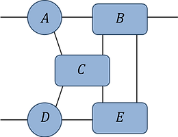
find the optimal contraction sequence for this network (assume all indices are of equal dimension d).

what is the leading order computational cost of this contraction? Express your answer as a power of d.

Ans: Contraction Sequence

Pb.1(b):

Index ordering conventions:

Network contraction:

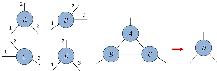
Pb.1(b)

Initialize rank-3 random tensors A, B, C (assuming all indices are dimension d = 20). Write code to evaluate the network contraction (using the specified index orders) in three different ways:

As a single summation over all internal indices using FOR loops.
As a sequence of binary contractions implemented using 'permute' and 'reshape'.
Using the 'ncon' routine.

Check that all three approaches produce the same output tensor D, and compare their respective computation times.

Ans: Python code

Problem Set 2:

PS2

Element-wise definition:

Pb.2: Tensor A is an order-4 tensor that we define element-wise as given above. Note that the difference between the MATLAB/Julia and Python definitions follows from the use of 1-based indexing in the former versus the use 0-based indexing in the latter, but it is still the same tensor between all three programming languages.

(a) Assume that indices i, j are of dimension d1 and indices k, l are of dimension d2 (with d2 < d1). How does the cost of taking the SVD across the indicated partition scale with d1 and d2?

(b) Generate the tensor A for d1 = 10 and d2 = 8. What is the norm ‖A‖? After computing the norm construct the normalized tensor: A' = A / ‖A‖.

(c) Take the SVD of A' across the indicated partition. Check that the square root of the sum of the singular values squared is equal to 1. Why is this the case?

(d) What is the effective rank r(Δ) of A' at Δ = 1e-4 ?

(e) Compute the truncation error ε of the restricted rank approximation r(Δ=1e-4) indirectly using the singular values as per Fig.2.4(c)

(f) Construct the optimal restricted rank approximation to A' via the truncated SVD. Compute the truncation error ε of this approximation and check that your answer is consistent with part (e).

(a) Cost is O(d1^2 ∙ d2^4), given as the larger matrix dimension times the square of the smaller matrix dimension.

(b) Norm: ‖A‖ ≈ 554.256

(c) Square root of the sum of the singular values squared is equal to the tensor norm, and we have normalized such that ‖A'‖ = 1.

(d) Effective rank r(Δ = 1e-4) = 3.

(e) Truncation error ε0 = 1.048e-5.

(f) Truncation error ε1 = 1.048e-5, consistent with the previous answer.

Ans:

Ans: Python code

Problem Set 3:

PS3

Fig.P3(a):

Fig.P3(b):

Pb.3: Consider the tensor network {A,B,C} → H of Fig.P3(a), with the element-wise definition of tensor A is given in Fig.P3(b) (note that the definition has been modified to account for 1-based indexing of MATLAB/Julia versus 0-based indexing of python). Define tensors B and C equivalently such that A = B = C, and assume that all tensor indices are of dimension d=12.

(a) Contract the network {A,B,C} to form the H tensor explicitly. Evaluate the norm ‖H‖.

Fig.P3(c):

Fig.P3(d):

(b) Use the truncated SVD to optimally decompose C into a rank χ=2 product of tensors, C → CL ⋅ CR, as depicted in Fig.P3(c). Contract the new network {A,B,CL,CR} to form a single tensor H1, as depicted in Fig.P3(d). Compute the truncation error ε = ‖H - H1‖ / ‖H‖.

Fig.P3(e):

(c) Starting from the original network {A,B,C}, transform tensor C into a center of orthogonality using the ‘pulling’ through approach based on the QR decomposition, obtaining a new network of tensors {A’,B’,C’}. Evaluate this network to a single tensor H' as depicted in Fig.P3(e), and then check that ‖H - H'‖ = 0.

Fig.P3(f):

(d) Repeat the truncation step from part (b) on the transformed tensor C' → CL' ⋅ CR', as depicted in Fig.P3(f), again keeping rank χ=2. Contract the new network {A',B',CL',CR'} to form a single tensor H1'. Compute the truncation error ε' = ‖H - H1'‖ / ‖H‖, and confirm that it is smaller than the result from (b). Why is this the case?

(a) ‖H‖ = 1.73e7

(b) Truncation error ε = ‖H - H1‖ / ‖H‖ = 9.45e-7

(d) Truncation error ε' = ‖H - H1'‖ / ‖H‖ = 1.06e-7. The truncation error from (d) is smaller since tensor C' was transformed into a center of orthogonality before truncation, which guarantees that the global truncation error is minimized.

Ans:

Ans: Python code

Problem Set 4 Solutions:

PS4

Fig.P4(a):

Pb.4: Consider the tensor H with the element-wise definition given in Fig.P4(a) (note that the definition has been modified to account for 1-based indexing of MATLAB/Julia versus 0-based indexing of python).

(a) Generate tensor H assuming all indices are dimension d = 6 and evaluate the norm ‖H‖. Define the normalized tensor H1 = H / ‖H‖

Fig.P4(b):

(b) Use a multi-stage decomposition to split H1 into a network of three tensors {A,B,C} while truncating to index dimension χ=6 as depicted in Fig.P4(b). Compute the truncation error ε = ‖H1 - H2‖, where H2 is the tensor recovered from contracting {A,B,C}.

Fig.P4(c):

(c) Make the appropriate change of gauge such that the A-B link becomes a center of orthogonality with a diagonal link matrix σ' as depicted in Fig.P4(d). What are the singular values in σ'? Check the validity if your gauge transformation by confirming that the singular values σ' in match those obtained directly from the SVD of tensor H2 across the equivalent partition.

Fig.P4(d-i):

(d-ii):

(d) Assume that the network T in Fig.P4(d-i) is in canonical form. Depicted in (d-ii) is the partial tensor trace of T with its conjugate network. Draw the simplified network that results from using properties of the canonical form to cancel tensors where-ever possible.

Ans:

(a) ‖H‖ = 6.389e2

(b) Truncation error ε = ‖H1 - H2‖ = 1.338e-7

(d) Canonical form implies the branch to the left of the A-D link annihilates to the identity with its conjugate, therefore the network simplifies as depicted below: